前篇:https://welts.xyz/2022/04/15/compute_map/.
这里我们关注简单计算图(即一个节点的值是一个浮点数,而不是矩阵)的实现。
基本图的构建
从基本的数据结构开始,定义基本计算图和计算图节点:
from random import randint

class NaiveGraph:

    node_list = [] # 图节点列表
    id_list = []   # 节点ID列表

    class Node:
        def __init__(self) -> None:
            # 生成唯一的节点id
            while True:
                new_id = randint(0, 1000)
                if new_id not in NaiveGraph.id_list:
                    break
            self.id: int = new_id

            self.next = list() # 节点指向的节点列表
            self.last = list() # 指向节点的节点列表
            self.in_deg, self.in_deg_com = 0, 0 # 节点入度
            self.out_deg, self.out_deg_com = 0, 0 # 节点出度
            NaiveGraph.add_node(self)

        def build_edge(self, node):
            # 构建self节点与node节点的有向边
            self.out_deg += 1
            node.in_deg += 1
            self.next.append(node)
            node.last.append(self)

    @classmethod
    def add_node(cls, node):
        # 在计算图中加入节点
        cls.node_list.append(node)
        cls.id_list.append(node.id)

    @classmethod
    def clear(cls):
        # 刷新计算图
        cls.node_list.clear()
        cls.id_list.clear()
这里的设计是嵌套类,且节点列表,加节点等方法都是类成员。这里的设计思想是,全局只有一个计算图,所有的操作都是在这个图上进行。这样操作的好处是,我们可以省去将节点显式加入计算图这一过程,这一步在节点的构造中已经隐式实现了。所以我们可以直接这样写
a = Graph.Node()
b = Graph.Node()
print(Graph.node_list)
发现Graph.node_list已经有两个节点了。这样能够更便捷地编写程序。
仿Tensorflow的节点属性
Tensorflow中有三种变量:
- 常量(Constant);
- 变量(Variable);
- 占位符(Placeholder)。
常量不存在导数,求导通常是对变量和占位符去求,而占位符通常是神经网络的数据输入口,我们借鉴TensorFlow,使用feed_dict方法对占位符进行赋值。我们模仿这样的设计方法,设计三个Node类的派生类:
class Constant(Node):
    def __init__(self, value) -> None:
        super().__init__()
        self.__value = float(value)

    def get_value(self):
        return self.__value

    def __repr__(self) -> str:
        return str(self.__value)

class Variable(Node):
    def __init__(self, value) -> None:
        super().__init__()
        self.value = float(value)
        self.grad = 0.

    def get_value(self):
        return self.value

    def __repr__(self) -> str:
        return str(self.value)

class PlaceHolder(Node):
    def __init__(self) -> None:
        super().__init__()
        self.value = None
        self.grad = 0.

    def get_value(self):
        return self.value

    def __repr__(self) -> str:
        return str(self.value)
注意到Constant节点的值是私有变量,表示不可更改,且没有梯度变量。
计算图的运算功能
上面的三种节点都是独立的,需要通过运算进行连接,所以我们定义Operator类:
class Operator(Variable):
    def __init__(self, operator: str) -> None:
        super().__init__(0)
        self.operator = operator
        self.calculate = NaiveGraph.operator_calculate_table[operator]

    def __repr__(self) -> str:
        return self.operator
注意到Operator节点,比如加法节点,乘法节点,也是有值有梯度的,所以Operator类可以继承自Variable。节点的运算符,我们用self.operator字符串存储,而self.calculate是self.operator对应的函数,比如,如果self.operator为"add",那么self.calculate是一个将self.last中节点值类加的函数。operator_calculate_table是一个字典,存储运算符字符串:运算函数的键值对:
from math import prod
from math import exp as math_exp, log as math_log
from math import sin as math_sin, cos as math_cos

operator_calculate_table = {
    "add": lambda node: sum([last.get_value() for last in node.last]),
    "mul": lambda node: prod([last.get_value() for last in node.last]),
    "div":
    lambda node: node.last[0].get_value() / node.last[1].get_value(),
    "sub":
    lambda node: node.last[0].get_value() - node.last[1].get_value(),
    "exp": lambda node: math_exp(node.last[0].get_value()),
    "log": lambda node: math_log(node.last[0].get_value()),
    "sin": lambda node: math_sin(node.last[0].get_value()),
    "cos": lambda node: math_cos(node.last[0].get_value()),
}
目前NaiveGraph支持四则运算,指数对数函数,正弦余弦函数。对于下面两个节点
constant = NaiveGraph.Constant
Variable = NaiveGraph.Variable

x = Constant(1, name='x')
y = Varialbe(2, name='y')
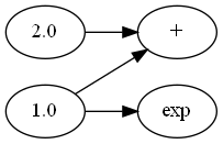
我们想计算加法,我们会新建一个加法节点,然后构建分别从x和y指向该加法节点的有向边:
add = Operator("add")
x.build_edge(add)
y.build_edge(add)
我们这里只建图,不计算,这是基于TensorFlow1的想法。计算步骤会在建图完成后交给前向传播来进行。至于一元运算,则是新建特定的运算节点,然后构建有向边:
exp = Operator("exp")
x.build_edge(exp)
至此为止我们构建了下面这样的计算图:
为计算图批量加入运算
如果对每一个运算都要重复地写上面的代码,未免过于麻烦,因此我们设计了三个函数模板:
- 一元函数模板;
- 二元函数模板;
- 可结合的二元函数模板。
先看一元函数:
@classmethod
def unary_function_frame(cls, node, operator):
    if not isinstance(node, NaiveGraph.Node):
        node = NaiveGraph.Constant(node)
    node_operator = NaiveGraph.Operator(operator)
    node.build_edge(node_operator)
    return node_operator
这里我们添加了一个前置操作,如果操作数的类型不是节点,而是一般的数字,比如
exp = NaiveGraph.exp(3.)
我们会将其转化为Constant节点。后面的操作我们在前面提到了,这里不再赘述。接着是一般的二元函数,类似的,我们会先将不是计算图节点的操作数进行类型转换:
@classmethod
def binary_function_frame(cls, node1, node2, operator):
    '''
    一般的二元函数框架
    '''
    if not isinstance(node1, NaiveGraph.Node):
        node1 = NaiveGraph.Constant(node1)
    if not isinstance(node2, NaiveGraph.Node):
        node2 = NaiveGraph.Constant(node2)
    node_operator = NaiveGraph.Operator(operator)
    node1.build_edge(node_operator)
    node2.build_edge(node_operator)
    return node_operator
最后是可结合的二元函数,针对的是加法和乘法:
@classmethod
def commutable_binary_function_frame(cls, node1, node2, operator):
    if not isinstance(node1, NaiveGraph.Node):
        node1 = NaiveGraph.Constant(node1)
    if not isinstance(node2, NaiveGraph.Node):
        node2 = NaiveGraph.Constant(node2)

    if isinstance(
            node1,
            NaiveGraph.Operator,
    ) and node1.operator == operator:
        node2.build_edge(node1)
        return node1
    elif isinstance(
            node2,
            NaiveGraph.Operator,
    ) and node2.operator == operator:
        node1.build_edge(node2)
        return node2
    else:
        node_operator = NaiveGraph.Operator(operator)
        node1.build_edge(node_operator)
        node2.build_edge(node_operator)
        return node_operator
这里的思想是,如果我们用上面一般的框架创建连续的加法节点,比如$1+2+3$,那么形成的计算图就是
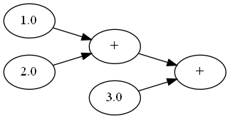
如果有$n$个节点连加,那么会形成$2n-1$个节点,但我们完全可以构建下面的计算图
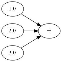
这样只需要$n+1$个节点就可以表达加法,适合这种结构的运算还有乘法。这是因为加和乘满足结合率:
\[(x+y)+z=x+(y+z)=x+y+z\\(x\times y)\times z=x\times(y\times z)=x\times y\times z\\\]在写好框架以后,每当新增一个一元or二元运算,我们只需要在NaiveGraph中加一个类方法,同时在函数表中注册对应的计算方法即可(实际上还有一项任务,即在导函数表中注册对应的求导方法),比如加法,减法和指数运算:
@classmethod
def add(cls, node1, node2):
    return NaiveGraph.associative_binary_function_frame(
        node1, node2, "add")

@classmethod
def sub(cls, node1, node2):
    return NaiveGraph.binary_function_frame(node1, node2, "sub")

@classmethod
def exp(cls, node1):
    return NaiveGraph.unary_function_frame(node1, "exp")
函数表中加上对应项即可。
为了让代码更简洁,我们实现了节点类的运算符重载,比如加法:
class Node:
    def __add__(self, node):
        return NaiveGraph.add(self, node)

    def __radd__(self, node):
        return NaiveGraph.add(node, self)
这样,下面的代码会直接创建上图的加法节点:
x = Variable(1, 'x')
y = Variable(2, 'y')
z = Variable(3, 'z')
s = x + y + z
前向传播
在构建好计算图之后,我们就可以求值。因为一个节点求值仅当它的操作数节点求值完成,因此使用拓扑排序进行这个过程。
@classmethod
def forward(cls):
    node_queue = [] # 节点队列

    for node in cls.node_list:
        # 入度为0的节点入队
        if node.in_deg == 0:
            node_queue.append(node)

    while len(node_queue) > 0:
        node = node_queue.pop()
        for next_node in node.next:
            next_node.in_deg -= 1
            next_node.in_deg_com += 1
            if next_node.in_deg == 0:
                next_node.value = next_node.calculate(next_node)
                node_queue.insert(0, next_node)

    for node in cls.node_list:
        node.in_deg += node.in_deg_com
        node.in_deg_com = 0
拓扑排序中,我们会不断删去入边,如果节点的入度为0,那么它就必须是求好值的。我们对入度是就地更改的,所以我们设计in_deg_com变量对修改的入度进行记录,在排序完成后再还原入度。
反向模式
我们在前面提到,反向模式相当于逆向的拓扑排序,也就是一个节点可以求导仅当它指向的节点的导数已经求好。
@classmethod
def backward(cls):
    node_queue = []
    for node in cls.node_list:
        if node.out_deg == 0 and not isinstance(
                node,
                NaiveGraph.Constant,
        ):
            node.grad = 1.
            node_queue.append(node)
    if len(node_queue) > 1:
        print('''
            计算图中的函数是多元输出,自动微分会计算梯度的和,
            如果要求指定输出的导数,应该是用backward_from_node。
            ''')

    while len(node_queue) > 0:
        node = node_queue.pop()
        for last_node in node.last:
            last_node.out_deg -= 1
            last_node.out_deg_com += 1
            if last_node.out_deg == 0 and not isinstance(
                    last_node,
                    NaiveGraph.Constant,
            ):  # 准备求导
                for n in last_node.next:
                    assert n.operator != None
                    last_node.grad += n.grad * cls.__deriv(n, last_node)
                node_queue.insert(0, last_node)

    for node in cls.node_list:
        node.out_deg += node.out_deg_com
        node.out_deg_com = 0
大体框架和前向传播相同,区别有:
- 我们设置出度为0的节点,即输出节点的梯度为1,因为$\partial f/\partial f=1$,其他节点的梯度都设为0;
- 如果计算图的节点有多个输出,那么求导时应当将这些输出对应的梯度相加,这也是为什么PyTorch等框架在每次反向传播前都需要将梯度清零的原因。
cls.__deriv是一个查表函数,表中是对应函数的导数:
@classmethod
def __deriv(cls, child: Operator, parent: Node):
    return {
        "add": cls.__deriv_add,
        "sub": cls.__deriv_sub,
        "mul": cls.__deriv_mul,
        "div": cls.__deriv_div,
        "exp": cls.__deriv_exp,
        "log": cls.__deriv_log,
    }[child.operator](child, parent)
具体的定义可以看源码。这里的问题是,如果是多元函数,比如
\[\pmb f(\pmb x)=(x_1+x_2,x_1-x_2)\]对应的计算图有多个输出(设$x_1=1,x_2=2$):
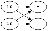
对1.0这个节点求导,导数会是两个输出对应的导数和$\dfrac{\partial f_1}{\partial x_1}+\dfrac{\partial f_2}{\partial x_1}$。但在这种情况下,这样的梯度加法是没有意义的,我们需要的是Jacobi矩阵,即
\[\begin{bmatrix} \dfrac{\partial f_1}{\partial x_1}&\dfrac{\partial f_1}{\partial x_2}\\ \dfrac{\partial f_2}{\partial x_1}&\dfrac{\partial f_2}{\partial x_2} \end{bmatrix}\]所以我们还设计了一个机制,即对某一个特定节点进行求导,它只有的入队代码和上面的反向传播有区别:
 @classmethod
def backward_from_node(cls, y):
    assert type(y) != cls.Constant, "常量无法求导"

    node_queue = []
    for node in cls.node_list:
        if node.out_deg == 0 and not isinstance(
                node,
                cls.Constant,
        ):
            if node == y:
                node.grad = 1.
            else:
                node.grad = 0.
            node_queue.append(node)

    while len(node_queue) > 0:
        ...
这里的机制是,我们只想求$\dfrac{\partial f_1}{\partial x_1}$和$\dfrac{\partial f_1}{\partial x_2}$,那么我们将$f_1$那个节点的梯度设置为1,$f_2$对应节点的梯度为0,那么从$f_2$流出的梯度将始终为0,不会对求导产生影响。我们为Variable类等提供这样的接口,这样的写法就挺像Pytorch了:
class Variable(Node):
    def backward(self):
        NaiveGraph.backward_from_node(self)
由此,我们可以实现Jacobi矩阵的求解:
@classmethod
def jacobi(cls, y_list: list, x_list: list):
    j = []
    for y in y_list:
        NaiveGraph.zero_grad()
        y.backward()
        j.append([
            x.grad if type(x) != NaiveGraph.Constant else 0.
            for x in x_list
        ])
    return j
例子
我们在https://github.com/Kaslanarian/PyAdNet/blob/main/naive_example.py中提供了三个例子。第一个例子是对函数
\(f(a, b) = a\times b + \log(a + b)\) 进行求值和求导,并与手动计算进行比较。结果
基于前向传播得到的c : 46.63906, 直接计算的c : 46.63906
基于反向传播得到的df/da : 4.07143, 手动求导得到的dfs/da : 4.07143
第二个例子是对一个多元函数
\[\pmb f(\pmb x)=(x_1+x_2+\log x_1,\frac{x_1}{x_2}+(x_1-x_2)^2)\]求Jacobi矩阵,并与手动计算结果比较:
NaiveGraph得到的Jacobi矩阵:
 [[2.0, 1.0], [-1.5, 1.75]]
手动求解的Jacobi矩阵:
 [[2.0, 1.0], [-1.5, 1.75]]
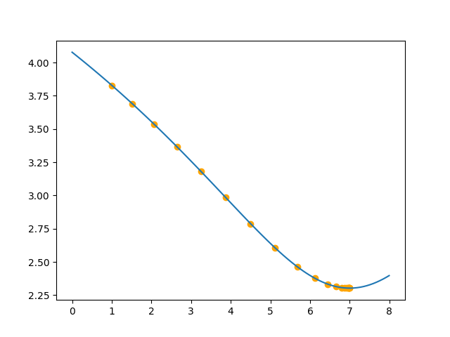
最后一个例子是对凸函数
\[f(x) = \log((x - 7)^2 + 10)\]进行梯度下降,求全局最优,初始点为1,效果如下:
总结
我们实现了效果不错的可自动微分的计算图,在此基础上,我们可以实现更复杂的,基于矩阵的计算图,从而实现神经网络。此外,将这种简单计算图移植到C++上,然后用Python调用去计算,也是笔者的一个想法。